This post focuses on Mixture of experts (MoE), which is used in modern models like Deepseek R1 and Qwen/Qwen3.5-35B-A3B. It's a way of reducing the number of active parameters per token (and per element in our batch) from the MLP layer and the performance difference is dramatic:
MoE is awesome. For local inference, which is typically batch size 1, it matters a lot how many parameters actually get used as they don't need to get transfered from (likely not high bandwidth) memory and we can save a lot of compute. For large-scale distributed inference, they also provide a more natural way to parallelize the models.
That A3B from Qwen/Qwen3.5-35B-A3B,
that's how many active parameters there are compared to the 35B total
parameters. To prevent ambiguity, we refer to the big MLPs as
dense layers and the layer itself we call FFN (feedforward
network) irregardless it being an MoE or dense MLP layer.
There is a lot to unpack about MoEs, so this blogpost will focus on small-scale inference setups, meaning one GPU or one or a two nodes, depending on the model you want to host. Hosting frontier MoEs like Deepseek R1 or Kimi K2 that approach 1T parameters is a whole different game, with many optimizations that will simply take too much effort to implement in our proof-of-concept inference engine. If you are interested in the economics of hosting those models, MoE Inference Economics from First Principles[1] is a good read.
So let's start with the simplest case, mixture of experts on one GPU, and move up from there.
Local inference on a single GPU
To understand the performance characteristics of MoEs, we first need to understand the architectural changes. Instead of a single MLP (two or three linear layers, depending on the exact model) per FFN, there is a router that selects \(k\) smaller MLPs, which are called experts. The router itself is also just a linear layer with a softmax and top-\(k\) to select the top \(k\) experts. We'll come back to the implementation of the router later.
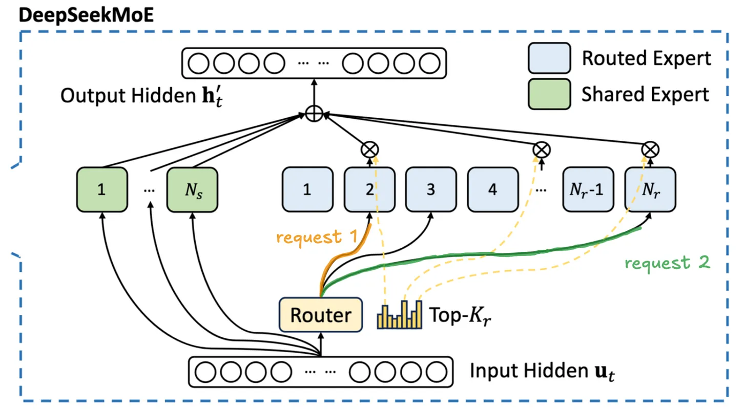
The difference in weight between the big, dense MLP and the smaller experts is quite staggering, the per-layer weight difference between a dense FFN and a single MoE expert is 9× for DeepSeek R1 (which has both in the same model), or about 16× for a Qwen3-30B-A3B expert vs a comparably-sized dense model's FFN. As a consequence, MoEs reduce the bandwidth cost of the MLP layer by significantly lowering the amount of data that needs to be moved from HBM to the streaming processors.
During decode, each token independently selects \(k\) experts. We simply our model by assuming uniform routing probability across all experts: each expert has an equal \(k/E\) chance of being selected per token. For a batch of \(B\) tokens, the expected number of distinct experts loaded from HBM follows from the coupon collector: the probability a specific expert is missed by all \(B\) tokens is \((1 - k/n_E)^B\).
\[\mathbb{E}[D(B)] = n_E \cdot \left(1 - \left(1 - \frac{k}{n_E}\right)^B\right)\]
Note that real models exhibit significant routing skew, so a small fraction of experts absorbs the majority of activations (see e.g. DeepSeek R1's expert distribution statistics[3]). Since skewed routing concentrates tokens onto the same popular experts, fewer distinct experts are touched at any given batch size than the uniform model predicts. Our uniform assumption therefore gives an upper bound on the number of distinct experts loaded from HBM, making the bandwidth savings for MoE layers we derive here conservative estimates.
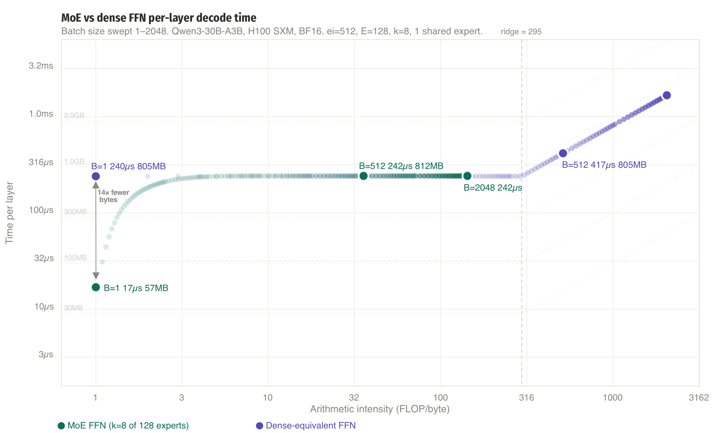
The demo below plots this for \(n_E = 128\) experts. At \(B = 1\) with \(k = 8\), only 8 of 128 experts are loaded from HBM, a 94% reduction in weight transfer compared to a dense FFN of equivalent capacity. Even at \(B = 128\), the expected number of distinct experts is around 113 rather than 128, thanks to the sublinear growth from the coupon collector effect.
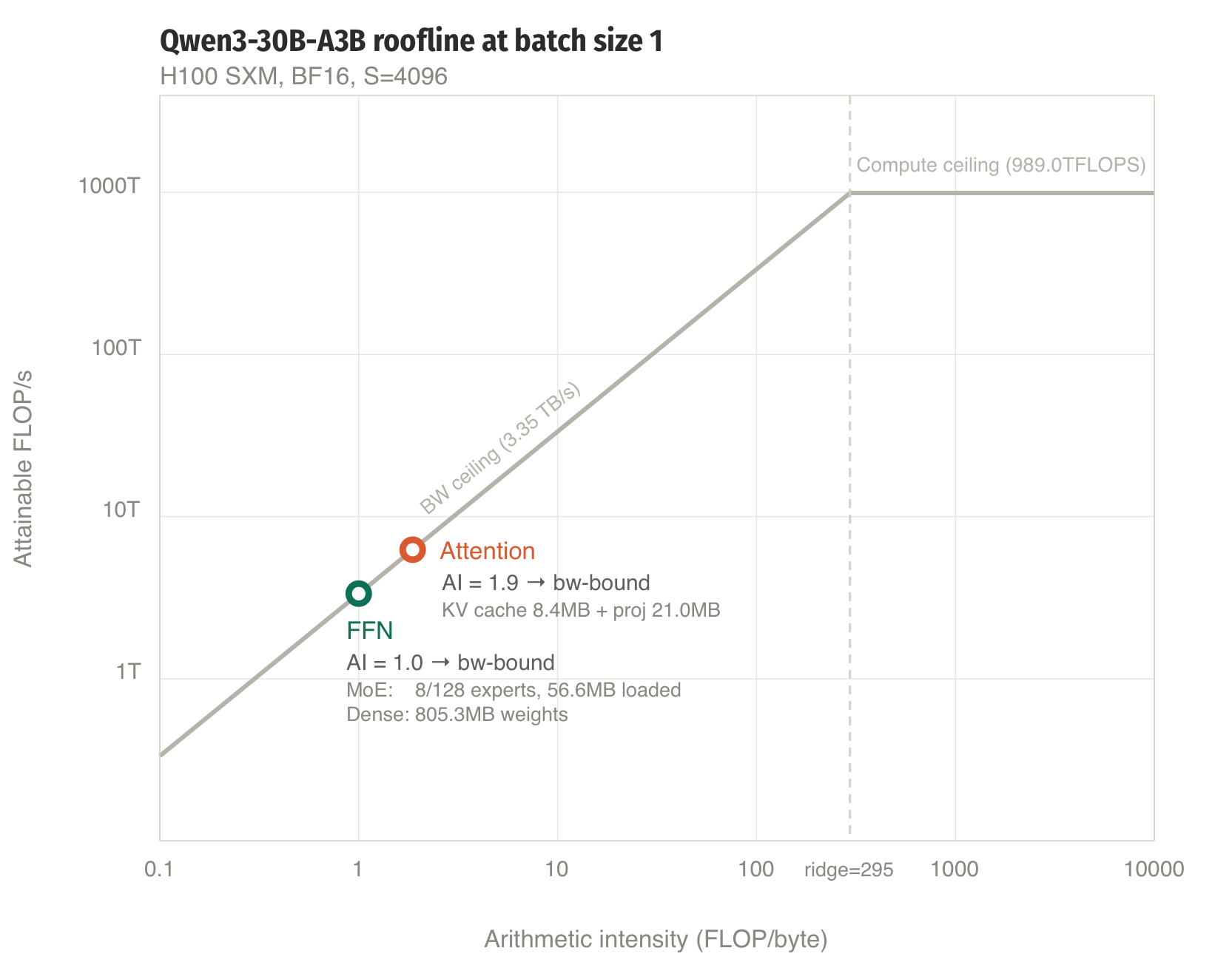
Now that we've looked at how many experts are loaded, we see that there are fewer distinct experts for small batches and for large batches. For instance, for B=1, we only have 8/128 experts that need to be loaded from HBW. That's a huge saving during autoregressive decode, as each generated token requires a full forward pass through the model. Whether a GPU spends that time waiting on HBM or doing useful math depends on (i) the arithmetic intensity of each operation and (ii) the active model size in bytes. And MoE models mix this up quite a bit.
We work through the numbers for Qwen3-30B-A3B on an H100 SXM (3.35 TB/s HBM bandwidth, 989 BF16 TFLOPS). The roofline's ridge point (the arithmetic intensity where you transition from bandwidth-bound to compute-bound) is:
\[\text{ridge} = \frac{989 \text{ TFLOPS}}{3.35 \text{ TB/s}} = 295 \text{ FLOP/byte}\]
Any operation with arithmetic intensity below 295 is bottlenecked by how fast we can read from HBM, not by how fast we can do matmuls.
| Symbol | Value | Description |
|---|---|---|
| \(d\) | 2048 | Model hidden dimension |
| \(L\) | 48 | Number of MoE layers |
| \(n_E\) | 128 | Routed experts per layer |
| \(n_s\) | 1 | Shared experts per layer |
| \(k\) | 8 | Top-k routed experts per token |
| \(d_{moe}\) | 512 | Expert intermediate size |
| \(h\) | 16 | Query heads (GQA) |
| \(h_{kv}\) | 4 | KV heads |
| \(d_h\) | 128 | Per-head dimension (\(d/h\)) |
| \(b_w\) | 2 | Bytes per weight (BF16) |
Each expert uses SwiGLU with three weight matrices: gate \([d_{moe}, d]\), up \([d_{moe}, d]\), and down \([d, d_{moe}]\). Small note that in the HF
checkpoints, gate and up are fused into gate_up_proj \([2d_{moe}, d]\) since they work on the same
hidden state inputs anyways. The parameter count per expert is:
\[P_e = 2 \cdot d \cdot d_{moe} + d \cdot d_{moe} = 3d \cdot d_{moe} = 3{,}145{,}728 \quad (6.3 \text{ MB in BF16})\]
Bytes.
Including the shared expert, the total bytes read are:
\[\text{bytes}_{\text{MoE}} = \left(\mathbb{E}[D(B)] + n_s\right) \cdot P_e \cdot b_w\]
FLOPs. Each of the \(B\) tokens activates \(k + n_s\) experts. For a single token (\(M = 1\)) through one expert's three SwiGLU matrices, that gives \(2 \cdot 3d \cdot d_{moe}\) FLOPs. A matmul \([M, K] \times [K, N]\) costs \(2MKN\) FLOPs, so:
\[F_{\text{MoE}} = B \cdot (k + n_s) \cdot 2 \cdot 3d \cdot d_{moe}\]
Arithmetic intensity. Dividing, the \(3d \cdot d_{moe}\) cancels:
\[\text{AI}_{\text{MoE}} = \frac{F_{\text{MoE}}}{\text{bytes}_{\text{MoE}}} = \frac{B \cdot (k + n_s) \cdot 2}{\left(\mathbb{E}[D(B)] + n_s\right) \cdot b_w}\]
In BF16 (\(b_w = 2\)), the factor of 2 from the FLOP count cancels the 2 bytes per weight, giving a clean expression that depends only on the routing, not on the model dimensions:
\[\boxed{\text{AI}_{\text{MoE}} = \frac{B \cdot (k + n_s)}{\mathbb{E}[D(B)] + n_s}}\]
At \(B = 1\): \(\mathbb{E}[D(1)] = k = 8\), so \(\text{AI} = 1 \cdot 9 / 9 = 1.0\). Interstingly, our arithmetic intensity is quite low, as it is exactly 1.0 and well below the ridge point, so we are hopelessly bandwidth-bound with our MoE FFN layer.
We'll come back to it later, but at \(B = 512\), our expected number of experts \(\mathbb{E}[D(512)] = 128 \cdot (1 - 0.9375^{512}) \approx 128\) (all experts loaded), so \(\text{AI} = 512 \cdot 9 \;/\; 129 = 35.7\). Both values are well below the ridge of 295: the MoE FFN is bandwidth-bound in both cases.
Dense-equivalent FFN comparison
A dense model with equivalent capacity would have a single FFN with intermediate size \(n_E \cdot d_{moe} = 65{,}536\). Its weights are always fully loaded regardless of batch size:
\[\text{bytes}_{\text{dense}} = 3d \cdot n_E \cdot d_{moe} \cdot b_w = 805.3 \text{ MB}\]
Every token uses the full weight, so:
\[\text{AI}_{\text{dense}} = \frac{B \cdot 2 \cdot 3d \cdot n_E \cdot d_{moe}}{3d \cdot n_E \cdot d_{moe} \cdot b_w} = \frac{2B}{b_w} = B\]
At \(B = 1\): AI = 1.0, which is the same as the MoE, but we are now loading 805 MB instead of 57 MB. The MoE advantage is purely fewer bytes, with a \(14\times\) reduction.
Again, we come back to the large-scale deployments with big batches later, but it's interesting to note already that at\(B = 512\), our AI = 512, which is well past past the ridge point. So the dense FFN becomes compute-bound. The MoE AI asymptotes to \(B(k + n_s)/(n_E + n_s) = B \cdot 9/129\), which is \(14.3\times\) lower than the dense AI of \(B\). This gap is structural: it's the ratio of total experts to active experts, and it never closes.
Bigger batches on a single GPU
At \(B = 512\), attention dominates at 73% of wall time. Each of 512 batch items reads its own KV cache, totalling 4.3 GB per layer — dwarfing the expert weights. The MoE FFN has lost its bandwidth advantage (all experts loaded), but its compute cost is still \(9/129 = 7\)% of the dense equivalent. The dense FFN, now compute-bound, would spend its time doing \(14\times\) more FLOPs per token. Total: 73.5 ms (~7.0K tok/s).
The MoE layer sits in an awkward middle on the roofline at large batch: too much data for the bandwidth (AI = 35.7 vs ridge = 295), too few FLOPs to be compute-bound. This is the regime where fused MoE kernels, expert parallelism, and quantisation matter most — each attacks the gap from a different angle.
Experimental validation: GPT-2 Large with 8 experts
We derived the roofline for Qwen3-30B-A3B with 128 experts. Now let's validate experimentally at a smaller scale. We take GPT-2 Large (\(d = 1280\), \(d_{ff} = 5120\), 36 layers) and convert it to Mixtral-style MoE by duplicating the FFN 8 times with top-2 routing. The weights are identical across experts — this doesn't matter for inference throughput (bytes are bytes), but it lets us verify correctness since the model should produce the same outputs as the original. The roofline principles carry over directly, just with \(n_E = 8\), \(k = 2\), \(d_{moe} = 5120\).
To understand where MoE sits on the performance spectrum, we compare four models:
| Model | \(d\) | \(d_{ff}\) | Layers | Params (approx) | Active FFN/token |
|---|---|---|---|---|---|
| GPT-2 Large (baseline) | 1280 | 5120 | 36 | ~774M | 5120 |
| MoE 8×, top-2 | 1280 | 8 × 5120 | 36 | ~5B | 2 × 5120 |
| Dense 5B (plausible) | 3200 | 8500 | 36 | ~5B | 8500 |
| Dense 5B (implausible) | 1280 | 40960 | 36 | ~5B | 40960 |
GPT-2 Large is the familiar baseline from the previous posts. The MoE model has the same total parameters as both 5B dense models, but only activates 2 of 8 experts per token. The plausible 5B dense model scales \(d\) to maintain a realistic expansion ratio (~2.7×). The implausible one keeps \(d = 1280\) and dumps all capacity into a \(32\times\) expansion FFN — the same pathology we flagged for Qwen3 above, but useful here because it isolates the FFN comparison with exactly the same residual stream as the MoE.
→ roofline predictions for all four models at B=1 and B=512
Naive MoE implementation
→ explain the nanoGPT-style implementation: routing logic, loop over experts, only compute active experts → code snippet of the MoE forward pass → note on weight duplication: copied 8× from GPT-2 Large FFN, verify outputs match original
Throughput comparison
→ benchmark all four models at B=1, B=8, B=64, B=512 (same methodology as previous posts) → at B=1: MoE should be close to GPT-2 Large (2× FFN work but same d for attention), both 5B dense models much slower → implausible 5B is especially bandwidth-hungry: 40K-wide FFN through 1280-wide residual stream → plausible 5B has larger attention cost too (d=3200), muddying pure FFN comparison → compare measured vs roofline predictions for all four
CUDA graphs
→ explain what CUDA graphs eliminate (kernel launch latency, CPU-GPU sync per expert) → what changes in the implementation → throughput numbers with CUDA graphs for the MoE model → speedup vs naive MoE, and how close to roofline we get now
Gap analysis
→ what's left on the table after CUDA graphs? → fused MoE kernels (e.g. Megablocks, vLLM grouped GEMM) — save for future post? → expert parallelism (TP>1) — save for future post? → quantisation — save for future post?
References
- Piotr Mazurek and Eric Schreiber, “MoE Inference Economics from First Principles”, Tensor Economics. ↩
- DeepSeek-AI, “DeepSeek-V3 Technical Report”, arXiv. ↩
- The SGLang Team, “Large-Scale Expert Parallelism”, LMSYS Blog. ↩